ARM Power Modelling

It is possible to model and monitor the energy and power usage of a gem5 simulation. This is done by using various stats already recorded by gem5 in a MathExprPowerModel; a way to model power usage through mathematical equations. This chapter of the tutorial details what the various components required for power modelling are and explains how to add them to an existing ARM simulation.

This chapter draws on the fs_power.py configuration script, provided in the configs/example/arm directory, and also provides instructions for how to extend this script or other scripts.

Note that power models can only be applied when using the more detailed “timing” CPUs.

An overview of how power modelling is built into gem5 and which other parts of the simulator they interact with can be found in Sascha Bischoff’s presentation from the 2017 ARM Research Summit.

Dynamic Power States

Power Models consist of two functions which describe how to calculate the power consumption in different power states. The power states are (from src/sim/PowerState.py):

UNDEFINED: Invalid state, no power state derived information is available. This state is the default.
ON: The logic block is actively running and consuming dynamic and leakage energy depending on the amount of processing required.
CLK_GATED: The clock circuity within the block is gated to save dynamic energy, the power supply to the block is still on and leakage energy is being consumed by the block.
SRAM_RETENTION: The SRAMs within the logic blocks are pulled into retention state to reduce leakage energy further.
OFF: The logic block is power gated and is not consuming any energy.

A Power Model is assigned to each of the states, apart from UNDEFINED, using the PowerModel class’s pm field. It is a list containing 4 Power Models, one for each state, in the following order:

ON
CLK_GATED
SRAM_RETENTION
OFF

Note that although there are 4 different entries, these do not have to be different Power Models. The provided fs_power.py file uses one Power Model for the ON state and then the same Power Model for the remaining states.

Power Usage Types

The gem5 simulator models 2 types of power usage:

static: The power used by the simulated system regardless of activity.
dynamic: The power used by the system due to various types of activity.

A Power Model must contain an equation for modelling both of these (although that equation can be as simple as st = "0" if, for example, static power is not desired or irrelevant in that Power Model).

MathExprPowerModels

The provided Power Models in fs_power.py extend the MathExprPowerModel class. MathExprPowerModels are specified as strings containing mathematical expressions for how to calculate the power used by the system. They typically contain a mix of stats and automatic variables, e.g. temperature, for example:

class CpuPowerOn(MathExprPowerModel):
    def __init__(self, cpu_path, **kwargs):
        super(CpuPowerOn, self).__init__(**kwargs)
        # 2A per IPC, 3pA per cache miss
        # and then convert to Watt
        self.dyn = "voltage * (2 * {}.ipc + 3 * 0.000000001 * " \
                   "{}.dcache.overall_misses / sim_seconds)".format(cpu_path,
                                                                    cpu_path)
        self.st = "4 * temp"

(The above power model is taken from the provided fs_power.py file.)

We can see that the automatic variables (voltage and temp) do not require a path, whereas component-specific stats (the CPU’s Instructions Per Cycle ipc) do. Further down in the file, in the main function, we can see that the CPU object has a path() function which returns the component’s “path” in the system, e.g. system.bigCluster.cpus0. The path function is provided by SimObject and so can be used by any object in the system which extends this, for example the l2 cache object uses it a couple of lines further down from where the CPU object uses it.

(Note the division of dcache.overall_misses by sim_seconds to convert to Watts. This is a power model, i.e. energy over time, and not an energy model. It is good to be cautious when using these terms as they are often used interchangeably, but mean very specific things when it comes to power and energy simulation/modelling.)

Extending an existing simulation

The provided fs_power.py script extends the existing fs_bigLITTLE.py script by importing it and then modifying the values. As part of this, several loops are used to iterate through the descendants of the SimObjects to apply the Power Models to. So to extend an existing simulation to support power models, it can be helpful to define a helper function which does this:

def _apply_pm(simobj, power_model, so_class=None):
    for desc in simobj.descendants():
        if so_class is not None and not isinstance(desc, so_class):
            continue

        desc.power_state.default_state = "ON"
        desc.power_model = power_model(desc.path())

The function above takes a SimObject, a Power Model, and optionally a class that the SimObject’s descendant have to instantiate in order for the PM to be applied. If no class is specified, the PM is applied to all the descendants.

Whether you decide to use the helper function or not, you now need to define some Power Models. This can be done by following the pattern seen in fs_power.py:

Define a class for each of the power states you are interested in. These classes should extend MathExprPowerModel, and contain a dyn and an st field. Each of these fields should contain a string describing how to calculate the respective type of power in this state. Their constructors should take a path to be used through format in the strings describing the power calculation equation, and a number of kwargs to be passed to the super-constructor.
Define a class to hold all the Power Models defined in the previous step. This class should extend PowerModel and contain a single field pm which contains a list of 4 elements: pm[0] should be an instance of the Power Model for the “ON” power state; pm[1] should be an instance of the Power Model for the “CLK_GATED” power state; etc. This class’s constructor should take the path to pass on to the individual Power Models, and a number of kwargs which are passed to the super-constructor.
With the helper function and the above classes defined, you can then extend the build function to take these into account and optionally add a command-line flag in the addOptions function if you want to be able to toggle the use of the models.

Example implementation:

class CpuPowerOn(MathExprPowerModel):
    def __init__(self, cpu_path, **kwargs):
        super(CpuPowerOn, self).__init__(**kwargs)
        self.dyn = "voltage * 2 * {}.ipc".format(cpu_path)
        self.st = "4 * temp"


class CpuPowerClkGated(MathExprPowerModel):
    def __init__(self, cpu_path, **kwargs):
        super(CpuPowerOn, self).__init__(**kwargs)
        self.dyn = "voltage / sim_seconds"
        self.st = "4 * temp"


class CpuPowerOff(MathExprPowerModel):
    dyn = "0"
    st = "0"


class CpuPowerModel(PowerModel):
    def __init__(self, cpu_path, **kwargs):
        super(CpuPowerModel, self).__init__(**kwargs)
        self.pm = [
            CpuPowerOn(cpu_path),       # ON
            CpuPowerClkGated(cpu_path), # CLK_GATED
            CpuPowerOff(),              # SRAM_RETENTION
            CpuPowerOff(),              # OFF
        ]

[...]

def addOptions(parser):
    [...]
    parser.add_argument("--power-models", action="store_true",
                        help="Add power models to the simulated system. "
                             "Requires using the 'timing' CPU."
    return parser


def build(options):
    root = Root(full_system=True)
    [...]
    if options.power_models:
        if options.cpu_type != "timing":
            m5.fatal("The power models require the 'timing' CPUs.")

        _apply_pm(root.system.bigCluster.cpus, CpuPowerModel
                  so_class=m5.objects.BaseCpu)
        _apply_pm(root.system.littleCluster.cpus, CpuPowerModel)

    return root

[...]

Stat Names

The stat names are usually the same as can be seen in the stats.txt file produced in the m5out directory after a simulation. However, there are some exceptions:

The CPU clock is referred to as clk_domain.clock in stats.txt but is accessed in power models using clock_period and not clock.

Stat dump frequency

By default, gem5 dumps simulation stats to the stats.txt file every simulated second. This can be controlled through the m5.stats.periodicStatDump function, which takes the desired frequency for dumping stats measured in simulated ticks, not seconds. Fortunately, m5.ticks provides a fromSeconds function for ease of usability.

Below is an example of how stat dumping frequency affects result resolution, taken from Sascha Bischoff’s presentation slide 16:

A picture comparing a less detailed power graph with a more detailed one; a 1
second sampling interval vs a 1 millisecond sampling
interval.

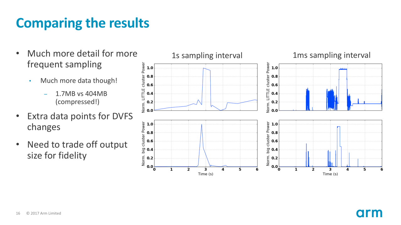
How frequently stats are dumped directly affects the resolution of the graphs that can be produced based on the stats.txt file. However, it also affects the size of the output file. Dumping stats every simulated second vs. every simulated millisecond increases the file size by a factor of several hundreds. Therefore, it makes sense to want to control the stat dump frequency.

Using the provided fs_power.py script, this can be done as follows:

[...]

def addOptions(parser):
    [...]
    parser.add_argument("--stat-freq", type=float, default=1.0,
                        help="Frequency (in seconds) to dump stats to the "
                             "'stats.txt' file. Supports scientific notation, "
                             "e.g. '1.0E-3' for milliseconds.")
    return parser

[...]

def main():
    [...]
    m5.stats.periodicStatDump(m5.ticks.fromSeconds(options.stat_freq))
    bL.run()

[...]

The stat dump frequency could then be specified using

--stat-freq <val>

when invoking the simulation.

Common Problems

gem5 crashes when using the provided fs_power.py, with the message fatal: statistic '' (160) was not properly initialized by a regStats() function
gem5 crashes when using the provided fs_power.py, with the message fatal: Failed to evaluate power expressions: [...]

These are due to gem5’s stats framework recently having been refactored. Getting the latest version of the gem5 source code and re-building should fix the problem. If this is not desirable, the following two sets of patches are required:

These can be checked out and applied by following the download instructions at their respective links.